Jiwoo Jung
The American International School of Vienna
jiwj07@gmail.com
PDF: https://shorturl.at/Sck1H
Abstract

Globally, billions of people continue to suffer from the contamination of water bodies with its scale and degree of impact ever-increasing. Yet, compared to the hundreds of thousands of rivers existing worldwide, the extent of studies done to analyze the water quality of rivers seem miniscule. As industrialization continues to predominantly contaminate the surface water of river flows, examination of water bodies becomes increasingly dire. This research compares and evaluates the industrial pollution within the Han River of South Korea and the Donau River of Austria, interpreting the independently collected data of water parameters of dissolved oxygen (DO), pH and total dissolved solids (TDS) as well as reviewing existing information regarding the two rivers, both quantitative and qualitative. Public data human population density (HPD) and air quality index (AQI) was utilized. Using cumulative air quality index (CAI) as the AQI for both rivers, All data revealed the exacerbating level of industrial pollution within the Han River in contrast to the Donau River experiencing manageable degree of contamination. The data were used to create matrices of Pearson’s correlation coefficients as well, of which the matrix cumulatively evaluating the data collected showed strong correlation between all pairs of the parameters examined, further validating the evaluation of the industrial pollution among both rivers. The data was used for training and testing 185 combinations of supervised machine-learning models in Python, applying various layers of feature selection. Ultimately, data from public databases were gathered to create linear models, nonlinear support vector regressor(SVR) models and model ensembles, applying k-fold Cross Validation while distinguishing between feature selection methods and dimensionality reduction techniques to ensure high accuracy.
Keywords: environmental science, ecology, river hydrology, industrial pollution, machine learning
1. Introduction
The rise in global pollution poses significant risks to both ecosystems and modern society. The contamination of rivers complicates the current cultural, economic, and political dynamics among human populations. Rivers foster unique biodiversity patterns that help mitigate the detrimental effects of human activities (Blanchet et al., 2020). Moreover, while rivers facilitate hydrologic, geomorphic, and ecological connectivity, they also play a crucial role in transferring organisms and sustaining biodiversity through the cycling of water. As global civilization increasingly urbanizes, the social connections among human populations become even more pronounced (Kondolf & Pinto, 2016). Additionally, river and environmental flows serve as a means to mitigate the impacts of anthropogenic activities, directly linking cultural values and lifestyles of communities while also protecting and restoring aquatic ecosystems (Anderson et al., 2019).
Water pollution is the contamination of water bodies, including rivers, lakes, oceans, groundwater, and even aquifers, by harmful substances, critically affecting the human population by placing human health, ecosystem, and the availability of water at risk (Mohamed, 2024). Affecting river flows as well, numerous aquatic systems around the world experience degradation as environmental flows become compromised despite its growing importance. Such degradation raises the urgency to maintain the water quality of rivers and environmental flows (Anderson et al., 2019). Since water is a fundamental aspect of the environment that provides important benefits for the human population, the management of water quality is essential: “Water is life without pollution, but death when it is polluted” (Igwe et al., 2017). The immediate call to action presents a crucial need to reduce the harm caused by water pollution to the ecosystem and human health. Among the two million people dying each year due to diarrhoeal illnesses, substandard sanitation of drinking water has led to approximately 90% of such deaths (Lin et al., 2022).
To discuss the pollutants of river pollution, anthropogenic activities such as agriculture appear to bring contamination and subsequent pollution to our varied ecosystems (Bashir et al., 2020). 38% of the streams extending across European nations are “significantly under agricultural pressure”; in the United States, agriculture is one of the primary sources of pollution within rivers and wetlands; agriculture has resulted in severe surface-water pollution and groundwater pollution of Chinese rivers (Bashir et al., 2020). These anthropogenic activities have resulted in the contamination of water sources through forms of bacteria and viruses, which are known as emerging pathogens due to their apparent virulence: pesticides, sludges, and sewages contaminated the soils of rivers and provided industrial discharges of chemicals and microelements, also becoming emerging pollutants of the environment and water bodies following industrialization (Mishra et al., 2023).
Among these sources of water pollution, industrial pollution is a leading cause within rivers:
globally, numerous people perceive and utilize water bodies as an “industrial dustbin” for discarding industrial effluents without bearing the extreme environmental cost (Igwe et al., 2017). It is the negative externality of industries avoiding corporate social responsibilities that continues to aggravate the problematic effect of industrial pollution. Sewage is the greatest volume of waste discharged into the aquatic ecosystems, of which the majority originate from industrial practices: as industries emit 80% of municipal wastewater into river bodies without filtration, millions of tons of heavy metals and toxic sludge eventually reach river bodies (Bashir et al., 2020). When exemplifying the case study on the Ganga River, bioaccumulation and biomagnification from industrialization and urbanization have placed human health and welfare in danger, highlighting the necessity for reducing industrial effluent released into the Ganga River (Roy & Shamim, 2020).
The assessment of water quality is significant in determining the level of pollution within an area and understanding its impacts; to calculate and quantify water quality, specific parameters of waters are measured. Conventionally, the water quality of a water body is considered to be accurately determined through a ‘water quality index’, or a WQI. In a study of 30 different WQIs and their characteristics, the indices are able to be organized into three categories: a fixed system of parameters, an open system where basic parameters are recommended but not limited to, and a mixed system in which consists of both basic and additional parameters (Sutadian et al., 2015). An observation could be deduced from the comparison that the nearly all WQIs commonly included parameters such as potential for Hydrogen (pH), Dissolved Oxygen (DO), Biochemical Oxygen Demand (BOD), Chemical Oxygen Demand (COD) and Total Solids (TS) (Sutadian et al., 2015). These physicochemical and biological parameters, according to multiple authors, vary seasonally. Moreover, anthropogenic activities, soil erosion and waste deposited into rivers have been identified as factors influencing one or more of the parameters, showcasing that a multitude of variables are able to affect the measurements of the parameters (Igwe et al., 2017). To interpret individually, Total Dissolved Solids (TDS), a particular type of TS, includes substances from domestic and industrial waste as well, resulting in a positive correlation with industrialization (Rusydi, 2018); the case study in Medlock River of Great Manchester, United Kingdom revealed the negative correlation between DO levels industrial land and a positive relationship with woodlands, whereas BOD had increased in concentration when wastewater was discharged into the river (Nguyen et al. et al., 2023); COD concentration had risen in the Anzali Wetland, Iran due to seasonal climate change (Tahershamsi et al., 2009); lastly, a decrease in the pH values could be observed in the Guadiamar River following the 1998 Aznalcóllar spill in Andalusia, Spain that raised the toxicity of the water, revealing a connection between pH and industrial discharges as well (M. Olías et al., 2005).
The Han River runs throughout South Korea and passes through multiple cities, from the riverhead Geomryongso, Taebaek to the Yellow Sea. It is a significant aspect of South Korea, supplying clean water to over 20 million people solely within Seoul, the nation’s capital (Lee et al., 2019). Occupying a watershed area of 26200 km2, the Han River has been straightened to be of 469.7 km in length for water control and presents a diverse ecosystem that should be maintained; yet the continual reduction in species such as the Korean eel (Anguilla japonica) indicates the threat faced by its ecosystem due to environmental degradation and pollution (Lee et al., 2019). The Han River is also extremely significant in the cultural context by providing aid throughout the development and settlement of the Korean civilization in addition to the economic benefits a long, controlled river provides (Lee et al., 2019). The management of the Han River is strictly managed by the South Korean government, as the river is an essential aspect of the nation. Subsequent to the industrialization of the nation, the government had recognized the importance of water quality management and undertook “multi-purpose dam” construction projects in the upstream region of the Han River while enacting five new regulations to protect the river (Shin et al., 2016). However, the management of the Han River has been increasing in difficulty as the water quality of the river body appeared to deteriorate. In particular, the eutrophication of the Han river is a substantial concern when managing the river’s water quality: the decline in BOD/COD ratio between 1986 and 2006 displays the increase in the proportion of recalcitrant organic matter, suggesting of a possibility of eutrophication of the river exacerbating(Shin et al., 2011). On the contrary, a decreasing trend of BOD levels could be observed due to the newly implemented sewage treatment facilities (Shin et al., 2011). Such evolved methods of regulation of the environment have begun to emerge in South Korea, invoked by the heightening of the pollution levels. As one of the selected procedures since the 1970s, Integrated Water Resource Management (IWRM) approaches are environmentally sustainable and considers human necessities (Hwang et al., 2020). Clearly illustrated by this study, methods of measuring and maintaining water quality become increasingly important as the consequential effects of environmental pollution become more drastic and complex.
The Donau River extends through numerous European nations, beginning in the Black Forest mountains of Germany and flowing until reaching the Black Sea. It is similarly significant to Austria as the second-largest river in Europe, stretching over a great distance of 2,845 km and critically influencing the ecological and economical landscape (Dávid & Madudová, 2019). Providing residence for diverse species of flora and fauna including endangered animals, the Donau river’s biodiversity appears to consist of over 320 avian species and a larger distinction among reptiles and amphibians (Vynokurova et al., 2023). The Danube River contributed to shaping the culture of Austria through various characteristics, allowing for “cultural, ethnic and political diversity” within the Donau River Basin (Schmid et al., 2023).
Similar to the Han River, the Austrian government provides management of the Donau River, but numerous organizations have implemented various ways of preserving it. The European Union’s enactment of the Water Framework Direction (WFD) exemplifies such involvement, proposing guidelines for a vast majority of European nations to follow (Stagl & Hattermann, 2015). Even so, as the urbanization of the nation continues, its environment continues to be damaged: within the last two centuries, the floodplain of the river has declined to less than 19% of the original size, demonstrating a decrease from 41605 km2 to 7845 km2 (Habersack et al., 2015). This decrease is detrimental, since most countries adjacent to the Donau River Basin generate over 45% of their hydropower through the Donau River Basin (Habersack et al., 2015). Furthermore, the contamination of the river’s water itself presents a further significant impact. The pollution of the river causes changes to the hydrodynamics of the river and restricts the spawning areas of a great number of species (Habersack et al., 2015).
Consistent sampling of water quality is extremely important in long-term safeguarding of river bodies, providing a quantitative measurement of the river’s pollution, consequences of industrial discharge, and the effect of urbanization. Numerous research emphasizes the importance of monitoring the water quality of rivers that reveals their current state. “Regular review of environmental effects of surface water pollution should be conducted by researchers to indicate the trend in pollutional loads of rivers, stream and lakes across the globe” (Igwe et al., 2017); “the evaluation of biological diversity have been recognized as an important national task to establish bio-sovereignty in the world” (Lee et al., 2019); “The paper emphasizes the importance of ensuring safe and clean drinking water through robust water treatment and monitoring systems” (Mohamed, 2024). Considering the implication above, this paper showcases a comparison of water quality and the effect of industrial pollution on the Han and Donau River, allowing important conclusions to be drawn from the two rivers located in hugely distinct settings. The research utilizes the parameters of DO, pH and TDS within the river bodies to evaluate the water quality of the Han and Donau River, supported with identified factors of industrial pollution.
2. Study area, materials and methods
2.1 Geographical setting
The data collection for the Han River was focused exclusively on the vicinity of Seoul. In a similar manner, this study gathered data from the region of Vienna. The selection of data collection sites was constrained by geographical challenges; thus, the Han and Danube Rivers were categorized into three segments: upstream, midstream, and downstream. The rivers’ streams were respectively trisected from the center of Seoul, South Korea and Vienna, Austria, with an approximate unit distance of 20 km between the data collection sites. Specifically, two sites of each stream were homogeneously selected to be directly opposite of one another as a means to account for variations in the collected data due to soil erosion, water flows, and geological settings. The sites were selected based on accessibility, as the majority of the river basin was limited in access. Hence, the selected sites slightly differed in terms of collecting DO, pH, and TDS. Since elevation is a primary variable that influences the physicochemical parameters of a river body, the altitude of the sites from sea level was recorded through a mobile application. The elevation of the data sites appeared consistent and there was minimal difference between the two rivers. Another factor to consider is the temporal setting of data collection. The DO data was collected during August and September of 2023; TDS and pH data were collected between the end of June and the beginning of August 2024. Thus, all data was collected during wet seasons, in which elements such as rain and temperature can cause volatility in the data reading that should be accounted for. The setting of data collection sites is summarized in Table 1. The specific geological area of data collection is displayed in Figures 1 and 2.
Table 1. Setting of data collection sites.

Figure 1. Map of DO data collection sites.
Figure 1. Map of DO data collection sites.

Figure 2. Map of pH and TDS data collection sites.
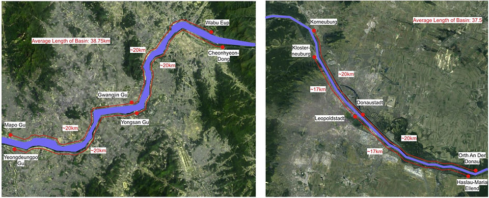
Footnote: Google satellite images used (Google Maps, 2019)
2.2 Data collection
The data was collected using a hand-crafted telescopic rod, which facilitated the gathering of 100 mL samples of surface water from the rivers at a depth of 5 meters at each data collection point. For measuring dissolved oxygen (DO), a Milwaukee Dissolved Oxygen Meter was employed, while pH and Total Dissolved Solids (TDS) were measured using Virph Digital Water pH TDS Temperature Meter. A digital water thermometer (CAS) was utilized to record the temperature of the samples. DO measurements were collected at one-minute intervals and recorded ex-situ within three days of data collection, resulting in 150 trials of data for each site. During the collection of pH and TDS data, values were consistently recorded by two sensors every 30 seconds for 75 trials each, minimizing fluctuations in the data and allowing for in-situ collection due to the shorter interval and reduced number of trials. The dates of sample and data collection were documented and are presented in Tables 2 and 3.
Table 2. Date of DO samples and data collection.
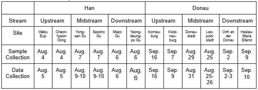
Table 3. Date of pH and TDS samples and data collection.

2.3 Modelling Methodology
In the study, three types of models were implemented in an attempt to identify the most accurate model for predicting industrial pollution based on various parameters: linear, support vector and ensemble. The Python library Scikit-Learn has been utilized for this research where multiple base models, feature selection methods and dimensionality reduction techniques are provided (Buitinck et al, 2013).
2.3.1 Linear Models
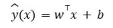
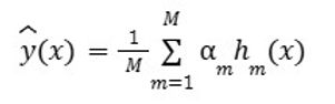
For linear models, six regressions were used as regressors/classifiers— linear regression, single-layer perceptron, lasso regression, ridge regression, elastic net regression and linear SVR. Linear models generally use the equation give below to adapt the model. Equation 1 describes a linear model where predictions are formed by summing weighted input features and a bias term. This structure assumes a direct, proportional relationship between variables and the output, making it foundational in machine learning. Often employed for regression and binary classification, the model’s simplicity supports interpretability and computational speed. However, its reliance on linearity limits its use in capturing complex patterns. Despite this, the linear model continues to serve as a baseline in empirical modeling, particularly when transparency and ease of implementation are prioritized over nonlinear predictive power.
Equation 1. Linear machine learning model equation

Linear regression is one of the most commonly utilized forms of ‘regression’ due to its simplicity. As the name suggests, the model is a best-fit linear line based on given data points, and the linear equation given below can be used to ‘predict’ a certain parameter. It typically uses Ordinary Least Squares (OLS) for optimization. Equation 2 outlines the Ordinary Least Squares (OLS) regression model, which estimates the linear relationship between a dependent variable and multiple predictors. Each coefficient reflects the marginal effect of a predictor, while the error term accounts for unexplained variance. By minimizing squared residuals, OLS yields efficient estimators under classical assumptions. This method remains central to empirical analysis across disciplines due to its clarity and interpretability. However, its performance may degrade under multicollinearity or heteroscedasticity, necessitating diagnostic evaluation and, in some cases, the use of regularization or transformation techniques to ensure validity.
Equation 2. OLS equation

Single-layer perceptron (SLP) is one of the earliest models used for classification, particularly in binary settings. As a basic neural unit, it operates on the principle of adjusting model weights based on prediction error during training. Equation 3 describes the learning rule used by the perceptron, which updates weights by adding a scaled version of the input vector if the predicted output does not match the true label. Although limited to linearly separable problems and unable to model complex decision boundaries, the perceptron remains a fundamental concept in the development of neural networks and modern deep learning systems.
Equation 3. SLP learning algorithm

Lasso regression expands upon the traditional linear regression approach by introducing a regularization component to promote sparsity. Specifically, the model incorporates an L1 penalty that constrains the sum of the absolute values of the coefficients. Equation 4 presents this loss function, where the penalty term effectively reduces certain coefficients to zero. This makes Lasso particularly useful in situations involving a large number of predictors, as it simultaneously performs variable selection and regression. However, the method may become unstable when predictors are highly correlated, as it tends to select one and discard others arbitrarily, limiting its robustness in such settings.
Equation 4. Lasso regression equation (L1 regularization)

Ridge regression offers an alternative to Lasso by using an L2 penalty to regularize the model’s coefficients. Unlike Lasso, Ridge does not zero out coefficients, but rather shrinks them toward zero, which can help mitigate overfitting and multicollinearity. As shown in Equation 5, the loss function penalizes the squared magnitudes of the coefficients, encouraging smaller and more balanced parameter values. This approach is particularly well-suited for situations where retaining all predictors is preferred, such as when interpretability is secondary to overall predictive performance.
Equation 5. Ridge regression equation (L2 regularization)

Elastic net regression combines the strengths of both Lasso and Ridge, using a weighted sum of their respective penalties to achieve a balance between sparsity and stability. The resulting loss function, shown in Equation 6, allows for variable selection while also addressing multicollinearity, which neither Lasso nor Ridge alone handle optimally. This dual-penalty approach is particularly advantageous in high-dimensional data settings where many predictors are correlated. By adjusting the weights of the L1 and L2 components, the model can be tailored to specific data characteristics, offering a flexible solution for complex regression tasks.
Equation 6. Elastic net regression equation (L1 + L2 regularization)

Linear Support Vector Regression (SVR) diverges from standard regression methods by introducing an epsilon-insensitive margin, within which prediction errors are not penalized. The prediction function, given in Equation 7, resembles that of other linear models but is optimized differently. Instead of minimizing squared error, SVR focuses on finding a function that fits the data while tolerating small deviations. This approach enhances robustness to outliers and small fluctuations in the data, making SVR particularly well-suited for tasks requiring high precision under bounded error margins, such as financial forecasting or control system modeling.
Equation 7. Linear SVR prediction function
2.3.2 Nonlinear Support-Vector Models
Nonlinear Support Vector Regressor(SVR) extends the linear SVR framework by incorporating kernel functions, allowing it to capture complex, non-linear relationships in the data. In this study, Nu- and Epsilon-SVR were utilized as nonlinear SVRs.
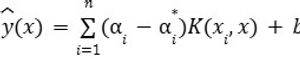
Equation 8 presents the prediction function for nonlinear SVR, where input features are mapped to a higher-dimensional space through a kernel, enabling linear separation in that transformed space. The prediction is determined by a weighted sum of support vectors and their corresponding coefficients, along with a bias term. This formulation allows SVR to model intricate patterns while maintaining robustness, particularly in applications involving irregular or highly variable datasets.
Equation 8. Nonlinear SVR prediction function
To implement nonlinear SVR, kernel functions are employed to implicitly project data into higher-dimensional spaces. Polynomial kernels, shown in Equation 9, capture curved decision boundaries by raising the dot product of input vectors to a fixed degree. The Radial Basis Function (RBF) kernel, described in Equation 10, is one of the most commonly used kernels, applying a Gaussian similarity measure that emphasizes local patterns. Equation 11 introduces the sigmoid kernel, which mimics neural activation functions and is occasionally used in network-based models. Equation 12 represents the cosine kernel, which compares the orientation rather than magnitude of vectors, making it suitable for text and high-dimensional sparse data. These kernels differ in their geometric assumptions and computational complexity, enabling model flexibility across diverse domains.
Equation 9-13. Nonlinear kernels

When training with nonlinear kernels, the resulting kernel matrix—also known as the Gram matrix—can be precomputed and stored to accelerate prediction, particularly when working with fixed training datasets. Equation 14 outlines how predictions can be made directly from the precomputed kernel matrix by applying the learned dual coefficients to the test set. This method is useful in large-scale applications or scenarios requiring repeated predictions, where runtime efficiency becomes a critical consideration. By leveraging the structure of the kernel matrix, the model maintains accuracy while improving computational performance.
Equation 14. Precomputed kernel matrix test prediction function
2.3.3 Model Ensembles
Rather than relying on a single model, ensemble methods combine multiple learning algorithms to produce a composite model that leverages the strengths of each individual component. The five model ensembles used in this study were Adaptive Boosting Regressor (ABR), Bagging Regressor (BR), Gradient Boosting Regressor (GBR), Histogram-based Gradient Boosting Regressor (HGBR) and Random Forest Regressor (RFR).
ABR combines multiple weak learners to form a stronger predictive model by emphasizing instances that are previously mispredicted. Equation 15 represents the ABR prediction function, where each weak learner contributes to the final output with an associated weight. The ensemble focuses sequentially on residual errors, progressively refining the model’s accuracy. ABR is particularly effective for data with complex error distributions, as it adapts to difficult cases by reweighting training samples. The overall effectiveness of ABR lies in its iterative error correction and capacity to reduce bias in underfitting base models. The choice of loss function in ABR governs how errors are penalized during model construction. Equation 16 defines a linear loss that directly penalizes the prediction error, offering simplicity but limited robustness. Equation 17 introduces a squared loss function, which amplifies larger deviations and is sensitive to outliers. Alternatively, the exponential loss in Equation 18 aggressively penalizes mispredictions and underpins the original AdaBoost algorithm, increasing the focus on incorrectly predicted samples. Each loss function alters how the ensemble adapts to errors, influencing both model sensitivity and convergence behavior.
Equation 15-18. ABR equations

BR aggregates predictions from multiple base models trained on bootstrapped subsets of the data. The prediction rule, described in Equation 19, computes the average output from all individual models, each contributing equally. This ensemble approach reduces variance without significantly increasing bias, enhancing model stability and performance on noisy data. Bagging is particularly useful in scenarios where single models overfit, as the averaging process tends to smooth out irregularities introduced by data fluctuations.
Equation 19. BR prediction equation
GBR iteratively builds models by fitting each new learner to the residuals of the previous ensemble’s predictions. Equation 20 formalizes this additive process, where the model is updated by combining the previous prediction with a scaled error-reducing function. This approach allows GBR to focus learning on areas where previous models underperformed. Its flexibility in optimizing different loss functions makes it widely applicable in structured data tasks, such as ranking, regression, and classification problems with nonlinearity and feature interactions. The effectiveness of GBR depends heavily on the loss function it optimizes. Equation 21 describes Mean Squared Error (MSE), the most common choice for regression due to its sensitivity to large errors. Mean Absolute Error (MAE), shown in Equation 22, treats all deviations equally, providing robustness to outliers. The Huber loss in Equation 23 merges both approaches by penalizing small errors quadratically and large errors linearly, making it suitable for noisy data. Equation 24 introduces the quantile loss function, enabling the model to predict conditional quantiles rather than mean outcomes, a valuable feature in forecasting intervals and risk-sensitive applications.
Equation 20-24. GBR equations

HGBR optimizes GBR by discretizing continuous features into histograms, enabling faster computation and memory efficiency. Equation 25 shows the update rule where each iteration adds a new learner to the model using a learning rate. Equation 26 presents the minimized loss function, often the quantile loss, which allows HGBR to perform robust regression under asymmetric error distributions. This design makes HGBR particularly efficient for large datasets while maintaining flexibility in handling skewed targets and heavy-tailed errors, a frequent concern in applied forecasting problems.
Equation 25-26. HGBR equations

RFR predicts outcomes by averaging the results of multiple decision trees trained on random data subsets and feature selections. Equation 27 defines this aggregation process, where each tree independently predicts an outcome and the ensemble combines them via averaging. RFR mitigates overfitting by introducing randomness and reduces variance through ensemble learning. Its capacity to model complex, nonlinear relationships without requiring extensive preprocessing has made it a preferred method in domains ranging from ecology to finance and clinical research.
Equation 27. RFR prediction equation

2.3.4 Feature Selection Methods
The five feature selection methods applied with the models were Chi-squared test, F-test/Analysis of Variance (ANOVA), mutual information test (MIT), Pearson correlation coefficient and recursive feature elimination (RFE).
The chi-squared test, introduced in Equation 28, is a statistical method used to determine whether observed distributions across categorical groups deviate meaningfully from what would be expected under independence. Commonly applied in contingency table analysis, it evaluates whether discrepancies in frequency counts arise by chance. This test is especially useful in classification contexts, where it can be employed to assess the relevance of categorical features. A higher value of the test statistic typically indicates stronger dependence between variables, providing a basis for feature selection or hypothesis testing.
Equation 28. Chi-squared test

Equation 29 defines the F-test, a foundational element in analysis of variance. This approach evaluates whether the variability explained by group differences exceeds the residual variation within those groups. When applied to continuous predictors segmented by a categorical outcome, the test helps identify variables with significant discriminatory power. It is especially effective in regression or classification pipelines, where selecting features that account for substantial between-group variance can improve model interpretability and performance.
Equation 29. F-test (ANOVA)

MIT, shown in Equation 30, offers a nonparametric approach for quantifying the shared dependency between variables. Unlike correlation-based methods, it captures both linear and nonlinear relationships, making it suitable for detecting complex associations. This measure is frequently used in feature selection tasks to identify predictors that provide substantial informational gain relative to the target. Its flexibility across data types has made it particularly valuable in domains with mixed or non-Gaussian distributions.
Equation 30. MIT equation
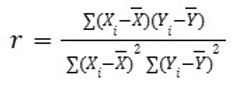
Equation 31 presents a statistical measure that quantifies the degree of linear association between two continuous quantities. By comparing their co-variability relative to individual variability, the metric reveals whether increases in one variable correspond to systematic changes in another. Frequently employed during the early stages of data analysis, it serves as a filter for identifying redundancies and collinear features. While limited to linear trends and sensitive to outliers, it remains one of the most widely used techniques for evaluating variable relationships.
Equation 31. Pearson correlation formula

The recursive feature elimination method, described in Equation 32, operates by systematically removing predictors that contribute least to model performance. At each iteration, the model is re-evaluated to determine the impact of each remaining feature. This approach enables the refinement of model complexity by prioritizing more informative variables. Widely used in high-dimensional contexts, it helps mitigate overfitting and improves generalization, particularly in models that rely heavily on input dimensionality.
Equation 32. RFE equation
2.3.5 Dimensionality Reduction Techniques
Lastly, seven dimensionality reduction techniques were used as the last process of the two-layer feature selection, consisting of Principal Component Analysis (PCA), Incremental PCA (IPCA), Sparse PCA (SPCA), Kernel PCA(KPCA), Truncated Singular Value Decomposition (TSVD), Factor Analysis (FA) and Dictionary Learning (DL).
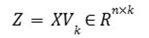
Principal Component Analysis (PCA), introduced in Equation 33, reduces data dimensionality by identifying new axes that capture the maximum variance within the dataset. The method begins with the construction of a covariance matrix, which represents the linear relationships among features. Equation 34 involves decomposing this matrix to extract directions that best explain variance. The final transformation, shown in Equation 35, projects the data onto these directions, generating a lower-dimensional representation that retains as much original information as possible. PCA is widely employed for visualization, noise reduction, and as a preprocessing step in machine learning pipelines.
Principal Component Analysis (PCA), introduced in Equation 33, reduces data dimensionality by identifying new axes that capture the maximum variance within the dataset. The method begins with the construction of a covariance matrix, which represents the linear relationships among features. Equation 34 involves decomposing this matrix to extract directions that best explain variance. The final transformation, shown in Equation 35, projects the data onto these directions, generating a lower-dimensional representation that retains as much original information as possible. PCA is widely employed for visualization, noise reduction, and as a preprocessing step in machine learning pipelines.
Equation 33-35. PCA equations

Incremental PCA (IPCA) is a computationally efficient extension of PCA that enables dimensionality reduction on streaming or large-scale datasets. Equation 36 defines how the data can be approximately reconstructed using a subset of principal directions. Equation 37 quantifies the reconstruction error, providing a measure of how much information is lost when reducing the number of dimensions. IPCA is particularly advantageous in scenarios where the entire dataset cannot be held in memory simultaneously, offering a trade-off between precision and scalability.
Equations 36-37. IPCA approximate data equations

Sparse PCA (SPCA) modifies standard PCA by introducing sparsity constraints, yielding principal directions that depend on fewer features. This enhances interpretability by identifying localized patterns in the data. Equation 38 describes the approximation of the original dataset using a reduced set of sparse components, while Equation 39 measures the resulting reconstruction error. SPCA is often applied in high-dimensional contexts such as genomics or text analysis, where standard PCA may obscure meaningful structure due to the inclusion of all features in every component.
Equations 38-39. SPCA approximate data equations

Kernel PCA (KPCA) generalizes PCA by enabling nonlinear dimensionality reduction through kernel methods. Equation 40 defines a matrix of similarity values computed in an implicitly transformed feature space, allowing the method to capture nonlinear relationships. The kernel matrix is then centered, as shown in Equation 41, to ensure that the transformed data retains zero mean. Equation 42 describes how data is projected within this feature space. KPCA is especially valuable when the underlying structure of the data is not linearly separable, making it suitable for tasks such as image processing and pattern recognition.
Equation 40-42. KPCA equations

Truncated Singular Value Decomposition (TSVD), as shown in Equation 43, produces a low-rank approximation of a dataset by retaining only the most significant singular components. This reduces dimensionality while preserving key structural information. A notable application of TSVD is Latent Semantic Decomposition (LSD), particularly in natural language processing, where it is used to extract hidden semantic relationships in term-document matrices. By projecting textual data into a reduced space, LSD captures underlying concepts that account for patterns in word usage, enabling improved retrieval and clustering. While TSVD assumes linear structure and lacks probabilistic interpretation, its effectiveness in compressing and revealing latent patterns has made it widely used in text analysis, information retrieval, and recommendation systems where data sparsity and redundancy are common.
Equation 43. TSVD LSE equation
Factor Analysis (FA), presented in Equations 44 and 45, models observed data as a linear combination of latent factors and noise. This generative approach assumes that underlying variables, which are not directly measurable, account for correlations among observed features. The covariance structure is explained through the contributions of these latent components and a diagonal error matrix. FA is frequently used in psychological testing, finance, and other domains where unobserved constructs are believed to drive observed outcomes.
Equation 44-45. FA equations

Dictionary Learning (DL), described in Equations 46–48, seeks to represent data as sparse combinations of elements from anoptimized basis set. The objective function minimizes reconstruction error while enforcing sparsity in the representation. Additional constraints are imposed to regulate the sparsity pattern across features or samples. This method is particularly powerful in signal processing, image compression, and sparse coding tasks, where the goal is to uncover compact, meaningful representations that facilitate both interpretation and efficient storage.
Equation 46-48. DL equations

3. Results and Discussion
3.1 Qualitative factors of industrial pollution
When perceiving the qualitative variables of industrial pollution, various factors contribute towards the overall contamination: for instance, a case study of the Karnafully River in Bangladesh identified pesticides, solid wastes and leakages as the primary pollutants of the river originating from nearby industries (Bhuyan & Islam, 2017). Another paper investigating the Ipojuca River in Brazil underscores the sugarcane factories raising the temperature of the water, organic acids exacerbating the river and excess potassium from fertigation fluids, resulting in the river being contaminated with biodegradable matter (Gunkel et al., 2006). Such inquiries highlight that a multitude of qualitative factors must be considered when examining industrial pollution.
In South Korea, the Han River has experienced the greatest number of contamination among the major rivers within the nation, accumulating to 283 cases between 2014 and 2018 (Jung, 2019). Over the course of the past five years, 5494873 m3 of sewage was produced daily by the 24263 active plants, of which 3823429 m3 was disposed in the Han River (Research Report - Research on the establishment of a conservation plan for the Han River Estuary Wetland Protection Area (20-24)). The sewage accumulates to be 11 million tons as wastewater being treated, which surpasses the legal restriction by 5 million tons of sewage (An, 2022). Such contamination also led to the Han River being ranked as the 43rd highest drug contaminated river among water bodies from 137 different countries (Cho, 2023). The declining water quality has been highlighted as a significant concern since the 1960s, when South Korea began industrialization (Kim & Seoul National University Graduate School of Environmental Studies, 2024). Such information establishes the Han River as a body of water highly polluted by industrial pollution.
Contrastingly, Austria’s Donau River seemingly suffers from industrialization to a minor degree: an evaluation from 2009 deemed 22% of the river as in ecologically good condition and 45% achieved good chemical status (Gasparotti, 2014). However, a study hypothesizing the independence of factories from the Donau River with continuing industrialization was disproven as the river’s water quality deteriorated with industries being able to transport their waste into the Donau River from a greater distance (Radu et al., 2020). This conclusion provides a counterclaim to the Donau River being generally less contaminated. Nonetheless, 97.7% of the nation’s water has been determined to be excellent in quality (International Commission for the Protection of the Danube River, 2022). The effort of the European Union to improve the water quality of the river has allowed the water to be safe for activities such as swimming (International Commission for the Protection of the Danube River, 2021). Hence, a multitude of evidence suggests the Donau River’s comparatively less extent of industrial pollution than the Han River.
3.2 Environmental variables
The surface water sample temperatures recorded during the collection of dissolved oxygen (DO) data in 2023 varied between 22.6°C and 29.2°C, with a maximum temperature fluctuation of 4.3°C at each site. Overall, the temperature showed a trend of either increasing or decreasing until reaching approximately 25°C. In 2024, during the collection of pH and total dissolved solids (TDS) data, the temperatures ranged from 24.5°C to 30.5°C. The maximum temperature variation observed per site was slightly higher than the previous year, measuring 4.7°C.
3.3 Physicochemical parameters
The mean, standard deviation(SD) and standard error of the mean(SE Mean) of the selected parameters for the water samples were presented in Tables 4 to 7. The DO value was narrowly within the tolerable range of 6.5 to 8 mg/L, the minimum being 6.660 mg/L and maximum being 7.709 mg/L; the pH varied between 7.496 and 7.643; lastly, TDS ranged from 83.912 to 196.628 ppm.
Tables 4-7. Statistical summary of river parameters.
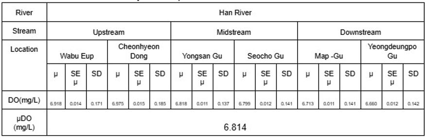

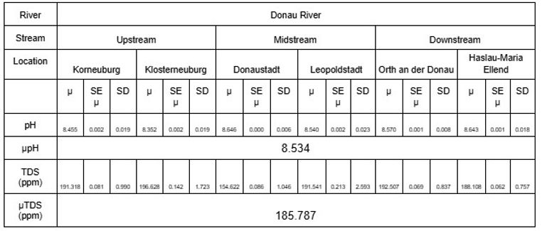
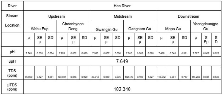
The statistical summary reinforces the claim that the level of industrial pollution in the Han River is severer than that of the Donau River. As conventionally known, low values of DO and TDS are associated with lower water quality and serious contamination of a river by signifying the lack of resources aquatic life consumes to survive, and vice versa; the Han River presents lower mean DO and TDS values of 6.814 mg/L and 102.34 ppm in comparison to the Donau River’s values of 7.502 mg/L and 185.787 ppm. Furthermore, pH represents the acidity of the water with lower values becoming more toxic, indicating contamination of the surface water; the mean pH value from the Han River of 7.649 is significantly lower than 8.534 from the Donau River. Both observations establish the Han River as being substantially polluted relative to the Donau River.
3.4 Human population density
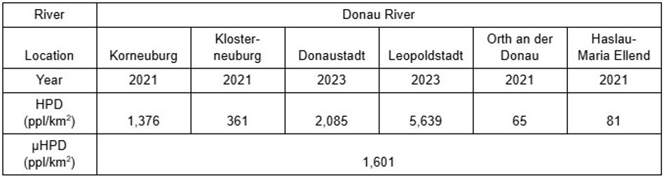
Human population density (HPD) measures the number of inhabitants within a defined area and serves as an indirect indicator of the level of urbanization and industrialization in different regions. Notably, population density provides a quantitative estimate of industrial pollution: a study conducted in the Weihe River of China revealed a relationship between HPD and industrial point-source sewage (Zhang et al., 2012). Similarly, HPD has been linked to industrial emissions in the Mediterranean regions, where areas characterized by high population density are considered highly susceptible to severe pollution (Acar & Mahmut Tekce, 2014).Thus, as HPD can be utilized as a possible method of evaluating industrial pollution, within the Han and Donau River, public data of HPD from and Austria Statistik was recorded in the data displayed in Tables 8 to 11. HPD values from 2021 were partly used as HPD during DO collection, since the Austrian government did not update the population of nearby regions of Vienna between 2021 and 2024.
Tables 8-9. HPD of South Korean and Austrian regions of DO data collection, 2021/2023

Tables 10-11. HPD of South Korean and Austrian regions of pH and TDS data collection, 2024


The tables show that HPD is naturally higher in regions located within South Korea’s capital Seoul and Austria’s capital Vienna. All within Seoul, Yongsan Gu, Seocho Gu, Gwangjin Gu and Gangnam Gu each displayed the highest HPD values of the recorded regions with respective values of 9,924, 8,617, 19,587, and 14,090 ppl/km2; similarly, Mapo Gu and Yeongdeungpo Gu are near the border of Seoul yet was highly populated. Situated in the center of Vienna, Donaustadt and Leopoldstadt also revealed HPD values of 2085 and 5639 ppl/km2 in 2023 as well as 2158 and 5722 ppl/km2 in 2024. The countryside regions of the two countries exhibited low values of HPD, ranging from 65 to 1160 ppl/km2. The overall HPD in South Korea appears to have been significantly higher in South Korea than Austria during both 2021 with Han River’s average HPD of 8417 and 10918 ppl/km2 in contrast to Donau River’s average HPD of 1601 and 1634 ppl/km2, further highlighting the likelihood that the Han River has experienced greater levels of industrial pollution than the Donau River.
3.5 Air quality index
The air quality index (AQI) provides information and insight into the contamination of air within a certain region by measuring specific pollutants within the air. Therefore, AQI serves as an indicator of pollution and potential health risks (Wu et al., 2021). Common pollutants that AQI measures are PM10, PM15, sulfur dioxide, and carbon dioxide (Cairncross et al., 2007). Each of these pollutants is harmful to human health and collected data of such parameters are utilized to create a cumulative value known as AQI. While the basic Air Quality Index ranging from 0 to 500 is most commonly used, certain regions in the world utilize different AQI types and metrics to evaluate the level of air quality and pollution within an area. Figure 3 provides the AQI descriptors of South Korea and the European Union (EU), which includes Austria (Wu et al., 2021).
Figure 3. AQI Descriptor of South Korea and EU
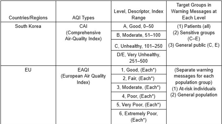
As the AQI demonstrates an aspect of pollution within an area, public AQI data from the World Air Quality Index Project was utilized, separating the region of data collection by provinces and averaging the AQI values of the data collection date from the nearest station to the data collection sites. As the EU does not specifically provide which index values are utilized for calculating EAQI, the AQI descriptor from South Korea was utilized. PM2.5 and PM10 were the two selected parameters that are the most common pollutants measured by AQI and other parameters differed per data collection station. The CAI was calculated by selecting the highest value and adding 50 if both PM2.5 and PM10 are included in categories C,D, or E; else, the highest value was selected as the CAI(AirKorea: Introduction to the CAI, 2022). Tables 12 to 15 summarize the recorded public data from DO data collection in 2023 and pH & TDS data collection in 2024.
Tables 12-13. AQI of South Korean and Austrian regions of DO data collection, 2023 (WAQI, 2008)

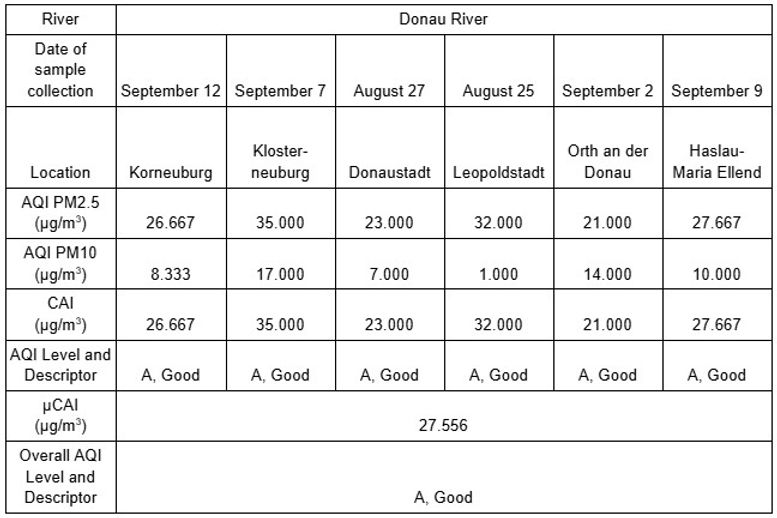
Tables 14-15. AQI of South Korean and Austrian regions of pH and TDS data collection, 2024 (WAQI, 2008)
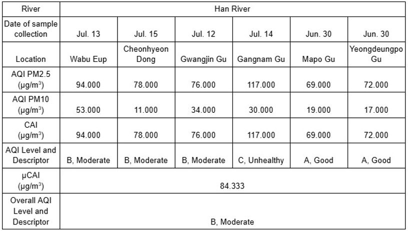

When interpreting the AQI data collected, unlike HPD, the CAI values revealed a general trend throughout the regions of the data collection sites instead of appearing to be significantly higher within the capitals. For instance, Wabu-Eup and Cheonhyeon Dong displayed higher CAI values between 56.000 and 94.000 μg/m3 during the data collection dates than Mapo Gu and Yeongdeoungpo Gu, which ranged from 51.000 to 72.000 μg/m3; the CAI values of Klosterneuburg was extremely inflated as well, 35.000 μg/m3 in 2023 and 31.000 μg/m3 in 2024, whereas Donaustadt displayed extremely clean air quality with values of 23.000 and 28.000. Such trends suggest that AQI is not directly associated with urbanized areas of population. However, this trend may be limited to the examination of small-scale areas, since the average CAI values of South Korean regions assessed the atmospheric condition as ‘B, Moderate’ and Austrian regions, which are less populated and industrialized than South Korea, as ‘A, Good’. Such overall results further support the possibility of the Han River being of a substandard level of industrial pollution in comparison to Donau River as more pollutants from industries are released into the air.
3.6 Relationship between physicochemical parameters
The data of the selected physicochemical parameters were utilized to reveal a bivariate correlation between each of the variables. Using the Pearson product-moment correlation coefficient, a correlation matrix of the mean physicochemical parameters of each river are presented in Tables 16 and 17. For HPD and AQI, the two datasets from 2023 and 2024 were averaged to be used for calculating the Pearson coefficients.
Tables 16-17. Pearson product-moment correlation coefficient matrix of physicochemical parameters of Han and Donau River
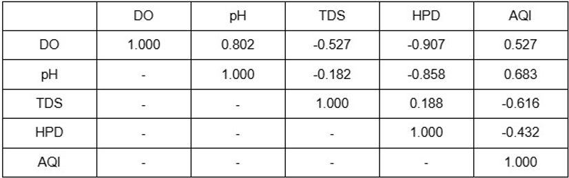

A general rule of thumb when interpreting Pearson correlation coefficients is the correlation being considered as strong when the magnitude of the coefficient is larger than 0.5, yet the correlation matrices appear to showcase no common relationships. While DO and pH has a high Pearson coefficient of 0.802 in the Han River, the pair of parameters display a negative trend with a coefficient of -0.858. Additionally, a strong correlation within a river is seemingly weak for the other: while pairs such as DO and HPD or pH and HPD showed extremely strong negative relationships of -0.907 and -0.858, the trends were not apparent from the parameters of the Donau River with coefficients of 0.254 and 0.084 for the respective pairs. Likewise, a moderately high coefficient of 0.527 between DO and AQI of the Donau River was opposed by a low coefficient of 0.255 of the same pair of parameters from the Han River. Hence, the two correlation matrices present the comparison between different sites of the identical river through the given parameters as possible yet imprecise.
To provide an overview of the relationship between the parameters in general, an alternate correlation matrix has been presented in table 18, cumulatively using the mean of the collected data throughout both rivers.
Table 18. Pearson product-moment correlation coefficient matrix of physicochemical parameters of both rivers
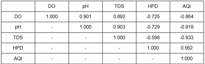
Unlike the previous correlation matrices, the cumulative table exhibits high Pearson correlation coefficients between all pairs of physicochemical parameters exploited, ranging from 0.691 to 0.896 in magnitude. Notable pairs of parameters demonstrating extremely strong relationships with each other are DO and pH with a coefficient of 0.901, DO and TDS with a coefficient of 0.8942, pH and AQI with a correlation of -0.918, and AQI and TDS with a correlation of -0.933. However, as the magnitude of the coefficient values are all above 0.562, all correlation between the parameters can be considered as strong. This difference in the strength of the correlation from the previous correlation matrices examining the parameters of each individual river signifies that the zero order relationships between parameters are strongly apparent when considering the correlation from a larger scale, specifically by cumulatively observing rivers instead of scrutinizing the changes between nearby data sites of each body of water.
The trends also align with the assumption of HPD and AQI serving as indicators of industrial pollution, and that they directly correlate with water parameters of nearby rivers. As DO, pH, and TDS displayed a negative Pearson correlation coefficient with the two indicators, all river parameters are inversely related to industrial pollution, with higher values of river parameters signifying lower levels of industrial pollution as well as higher water quality and vice versa. Consequently, all other pairs of parameters display positive relationships. Since all parameters had concluded the Han River’s high level of contamination relative to the Donau River, the strong relation between all parameters displayed through the Pearson correlation matrix displays this conclusion as highly reliable. This conclusion also aligns with the trend of the Han River seemingly experiencing greater industrial activities than the Donau River, proposing industrialization as a primary variable affecting the two rivers’ water quality and level of pollution. Lastly, the correlation matrix provides all five parameters examined as appropriate for comparing the level of industrial pollution among different rivers.
3.7 Machine-learning modelling of collected data
While the relationship between the five parameters (DO, pH, TDS, HPD, AQI) has been identified, the paper’s objective of providing individuals an accessible and affordable method of measuring industrial pollution remains unattained. DO, pH and TDS data can be collected from cheap meters with acceptable margin of error, while HPD is frequently calculated by the government with nearly perfect accuracy; however, AQI is a value that is limited in public data due to the low number of data collection centers yet requires advanced tools costing up to thousands of dollars to accurately measure air pollution, resulting in data being low in accuracy and even inaccessible in some areas.
Hence, to resolve this issue while also exemplifying the possibility of applying the paper’s finding about the parameters, various computerized models estimating AQI based on data of other parameters were created. Since individuals would be using such models to estimate AQI for a specific river, the data set was split into the data of the Han and the Donau River, using the first set to train the model and second set to compare the predictions and actual values. As the study researched for AQI and HPD of years 2023 and 2024 since the river parameters were collected during both years, the mean AQI and HPD values were utilized as the testing set. The built-in standard scaler within the library was utilized to allow the variables to be calibrated and balanced by the models.
3.8 Accuracy of the models
In addition to the five base models and the three feature selection methods/dimensionality reduction techniques mentioned in the methodology, up to two layers of feature selection were applied to create the models. Models in which four or more features are selected were removed because feature selection is intended to narrow down the total number of parameters used to predict AQI (CAI was once again selected as the type of AQI for predictions). For a similar reason, 2-layer models in which the second layer selects the same number of features as the first layer or more were not considered as well. Since little to no prior research of modelling these parameters had been conducted for these parameters, combinations of feature selection methods (PCA, RFE, UNI) and base regressors/classifiers (Linear, SLP, Lasso, Linear SVR, RFR) mentioned above were tested, resulting in a total of 185 models. The results for all models are given in the Appendix. The paper tests various computerized models, using Root Mean Squared Error (RMSE) and mean absolute error (MAE) between the predicted values and actual values of AQI to evaluate its accuracy. The mean, maximum, minimum and second smallest RMSEs as well as MAEs of the tested models are displayed in Tables 19 and 20.
Table 19. Mean, minimum and maximum RMSE of tested models

Table 20. Mean, minimum and maximum MAE of tested models

Generally, the RMSE and MAE of all models were generally quite high. The RMSE ranged significantly from 30.324 (Lasso Regression) to 79.902 (Linear-PCA3-RFE2 and Linear-PCA3-UNI2 models); the MAE varied within a similar range from 26.014 (Lasso Regression) to 78.433 (Linear-PCA3-RFE2 and Linear-PCA3-UNI2 models). Based on both errors, the Lasso Regression model without any feature selection layers appears to be the most accurate. The RMSE of the predictions using Lasso Regression was 30.324, slightly smaller than that of Linear Regression, 30.542. Likewise, its MAE of 26.014 was similar to that of the Linear Regression of 26.206. Lasso Regression’s MAE was 61% of the mean MAE of 49.806 and the rMSE was 53% of mean rMSE 49.131, showing the significant accuracy of its programs compared to other models. Hence, although the models seem inaccurate and insignificant for estimating AQI using the four parameters, the SVR-PCA2-RFE1 model can be considered as providing AQI predictions that are of acceptable accuracy. Through this model, the level of industrial pollution within an area will be able to be tested affordably, raising interest for the impacts of industrial pollution and ultimately motivating individuals to advocate against this destruction of the environment.
3.9 Identifying cause of inaccurate predictions
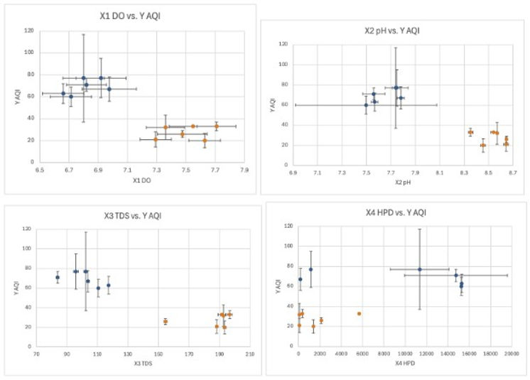
The large errors of the models’ predictions were expected due to a number of limitations regarding the parameters and data. Firstly, AQI itself is a very volatile parameter since there is an extensive number of fast-changing uncontrolled variables affecting it, such as strength of wind, rate at which pollutants are released into the air or type of weather; in conjunction with the restrictive amount of AQI collection sites and data available, the inaccuracy within the data set complicates the process of predicting AQI data. Another possible reason is the smaller number of data collection sites themselves, as 12 sites signifying 6 data points used for training and 6 for testing the model, which is an extremely small amount. Likewise, the limited number of parameters presumably restricted the number of patterns the model was able to identify, increasing its inexactness. However, the most influential factor causing the imprecision of the models is likely the clustering of data based on rivers, since the paper has already identified that the river data is clustered together and hence requires data from more rivers (collected with the same methodology) to accurately model the general relationship between the parameters and industrial pollution throughout rivers. As data is clustered, datasets from more than one river are required to form a semi-accurate regression that identifies the trends throughout each river instead of being specific to one river. This major limitation can be resolved through a machine-learning approach where online databases of data can be implemented to the computerized models, which would significantly increase its accuracy. The clustering is demonstrated within the scatter plots provided below in figures 4 to 7, in which the plots to the left are based on data from the Han River and plots to the right are of the Donau River.
Figures 4-7. Scatter plots of each parameter against AQI demonstrating clustering of data (Han river dataset in blue, Donau river dataset in orange)
3.10 Analyzing possibility of improving the model
To consider whether an increased number of rivers within the dataset has a possibility of improving the model’s predictions of the AQIs, the clustering must be present throughout the analysis of the model, allowing the model to create a regression passing through every cluster. While analyzing the clustering of data for every model would be ideal, creating and examining scatterplots of 185 combinations of models and feature selections would prolong and complicate the study to a great extent. Hence, the scatterplots of data after normalization and applying PCA feature selection were selected for analysis as such scatterplots are apt for visualization. The scatterplot of initial data is provided below alongside that of normalized data in figures 8-9.
Figures 8-9. Scatterplots of initial and normalized data
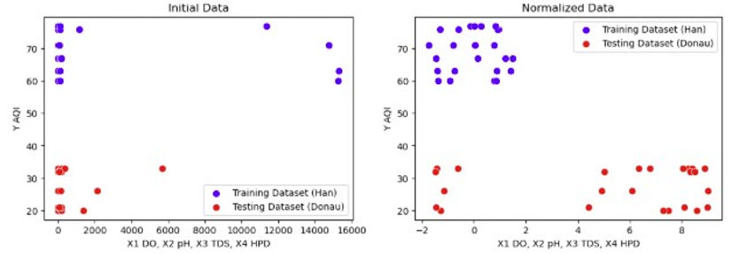
As demonstrated by the clear difference between the two figures above, the clustering of the data from the Han and Donau river appears more evident: while four outliers from the training dataset (Han river) dataset were initially located in the upper right-hand corner, the outliers became part of the cluster after normalizing the data. Contrastingly, new outliers appeared among the testing dataset (Donau river) although of a less extreme degree than the previous outliers, suggesting the limitations of clustering of data with only normalization. For a more detailed analysis of the outliers, scatterplots labelled with specific parameters are provided in figures 10-11.
Figures 10-11. Labelled scatterplots of initial and normalized data
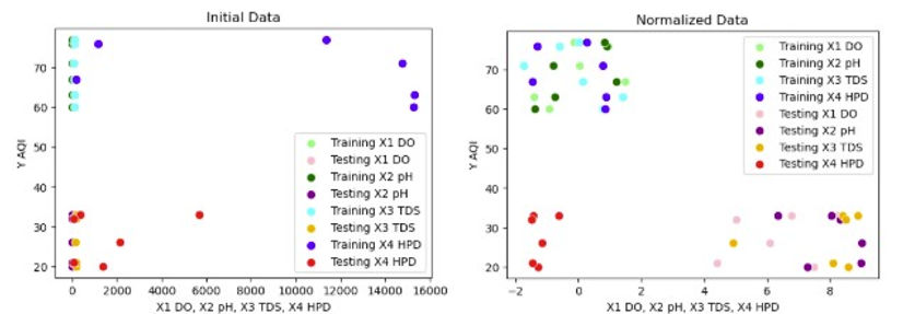
As noticeable through the scatterplots, the outliers from both rivers were due to HPD data from both rivers. This observation suggests that models of greater datasets can predict AQI with a relatively high accuracy if feature selection layers were applied and effectively removed HPD data. However, this is based on the assumption that HPD data of all rivers does not complement the overall trend of the dataset in comparison to DO, pH and HPD, which cannot be justified with data from only two rivers. Subsequently, the scatterplots after applying PCA were analyzed to investigate if HPD data was removed from the testing and training dataset.
Figures 12-14. Scatterplots of normalized data after applying PCA

After PCA was applied, the assumption of HPD being removed from the dataset was proven true, further justifying the possibility for the machine-learning model being able to predict AQI more accurately with greater datasets: comparing with scatterplot of the normalized data, the outliers were removed after applying PCA of 3, 2 and 1 components. The clustering is most prominently evident in PCA2, leading to the prediction that selecting two features would provide the most accurate model after more data is added.
3.11 Model with increased dataset
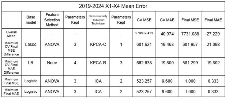
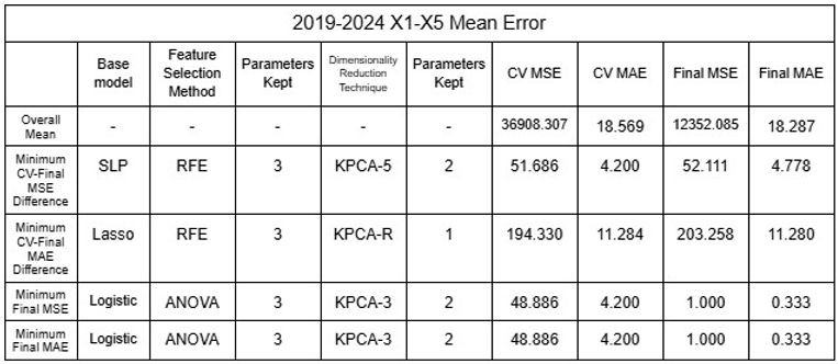
After identifying that the inaccuracy of the model was likely due to the clustering of data public data was utilized to increase the dataset of rivers the model could be trained and tested with [16-19]. Two different sets of data were tested: 2015-2024 and 2019-2024, each of 65 and 44 rivers from various nations around the world. Additionally, because total population appeared to show correlation with the predictions when testing, additional datasets were used with population as X5 variable. Using the mean values and considering each river as a plot, the dataset was shuffled with the models to test the model’s reliability by randomizing the large number of data it uses for training and testing. All models (regressors and classifiers) discussed above were utilized and dimensionality reduction techniques were distinguished from feature selection methods and applied as the last layer of the model to ensure accuracy by undergoing noise reduction with feature selection before changing interpretability with dimensionality reduction; this procedure allowed 11,632 different permutations to be tested, accumulating to be over 45,000 for all datasets combined. RFE was not applied to NuSVR, Epsilon SVR, BR or HGBR because such regressors do not rank features automatically, which is required to implement RFE. K fold Cross-Validation was also implemented to increase accuracy of model, and 5 folds were conducted for each permutation. As the data was randomized, five trials were conducted to confirm its accuracy. The results of the minimum errors are provided in Tables 21 to 32.
Tables 21-24. Mean and Standard Deviation RMSE and MAE of 2015-2024 and 2019-2024 linear models


Tables 25-28. Mean and Standard Deviation RMSE and MAE of 2015-2024 and 2019-2024 SVR models
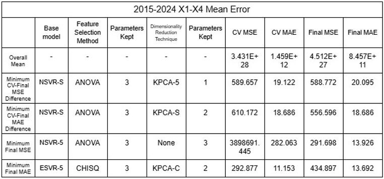

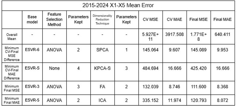
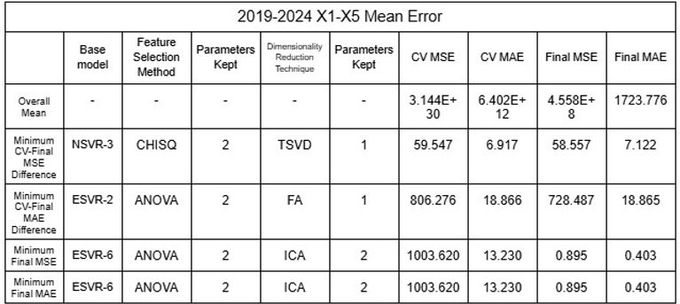
Tables 29-32. Mean and Standard Deviation RMSE and MAE of 2015-2024 and 2019-2024 model ensembles

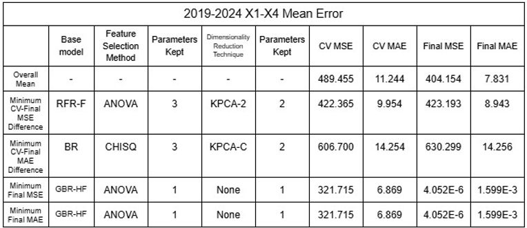


The low values of mean error clearly indicates that the models using the large datasets demonstrated a significant degree of accuracy. Furthermore, NSVR-3 with CHISQ2 and TSVD1 or RFR-F with RFE2 and KPCA1-6 exemplify models of minimal difference between average cross validation error and final error after testing, showing that models have not been overfitted and are reliable. While nonlinear SVRs appear to be the most accurate with minimum MSE and MAE of 0.895 and 0.403, different models displayed above can be selected based on the objective of the user, such as minimizing CV-Final error difference or prioritizing MAE over MSE.
4. Limitations
4.1 Limitations of data collection
A notable limitation of the case study is the considerable variation observed between data points. The fluctuations in environmental variables, such as sample temperature, were more pronounced in situ due to the volatile conditions present at the site. In contrast, the physical data concerning dissolved oxygen exhibited significant discrepancies when compared to the pH and TDS data, likely as a result of the data being collected ex-situ. Additionally, the differing midstream data collection sites in 2023 and 2024, while accounting for the distance between locations to a certain extent, led to variations in the population density values for that section.
4.2 Limitations of data modelling
The finding of feature selection increasing the accuracy of the machine-learning models is contradictory to the most accurate model trained with Han and Donau River being Lasso regression trained using normalized data without feature selection layers. However, this counterclaim can be easily resolved since all models showcased high degrees of errors and the selected model is still inaccurate nonetheless.
5. Conclusion
This study aimed to examine the industrial pollution among the Han River of South Korea and the Donau RIver of Austria, collecting data on DO, pH and TDS as parameters of the rivers’ surface water. The study also correlated various parameters to explore relationships and identify reliable indicators, using the Pearson’s Correlation Coefficient matrices to interconnect the physically collected data alongside public data of HPD and AQI used as additional parameters. Qualitative evaluation of the severity of industrial pollution among both rivers was conducted as well by identifying variables such as the amount of sewage from factories being discharged into the rivers or consequences of urbanization, which revealed the significant degree at which industrial pollution occurs in South Korea that affects the Han River in comparison to Austria and the Donau River. The data of river parameters, HPD and AQI all aligned with general trends of the Han River being significantly more polluted than the Donau River through data sites demonstrating comparatively high DO and TDS values, low pH values, high HPD values and high AQI values (CAI used as type of AQI), aligning with the qualitative assessment. The correlation matrices showcased asymmetrical patterns when parameters from data sites within the river were compared. However, when compared cumulatively, all pairs of parameters displayed strong zero order relationships with the magnitude of the Pearson coefficient ranging from 0.691 to 0.903. The results present the interconnected relationship between the five parameters examined and the viability of them as indicators of industrial pollution when comparing multiple rivers. The data analysis models created based on such relationships identified between parameters allow for predictions of AQI data with varying accuracy. This ability to predict AQI removes the need for expensive measurement devices for identifying the level of industrial pollution, allowing for the general audience to access or obtain such data and raising awareness for the global issue of climate change. Similarly, other researchers can utilize the model(s) to estimate AQI based on other interconnected parameters, broadening their scope of research. The study affirms that the Han River as experiencing severe industrial pollution whereas the Donau River is being contaminated to a tolerable degree, supported by the collected data of physicochemical parameters from the rivers’ surface water, HPD and AQI values of the data sites, and the multitude of factors affecting the rivers’ industrial pollution. The study also establishes Lasso Regression models as appropriate for predicting AQI as AQI with some errors, the RMSE and MAE being comparatively low values of 30.324 and 26.014, respectively. In the near future, implementing a machine-learning approach using databases of data is also possible, allowing for improvement in its accuracy as well as possibly suggesting different models to be more suitable for predictions. Lastly, ESVR-6 applying ANOVA2 and ICA2 appears to be the most accurate model with final MSE and MAE of 0.895 and 0.403, but as models such as NSVR-3 with CHISQ2 and TSVD1 or RFR-F with RFE2 and KPCA1-6 showcase smaller difference between average Cross-Validation and final error, different models can be selected for different purposes with the majority of models ensuring high accuracy in all categories nonetheless.
6. Acknowledgements
This research was conducted individually, but I would like to acknowledge Leon Plakolm as my research mentor that supervised the process of publishing this paper.
7. Data Availability
Data will be made available on request. Similarly, code used for testing models can be requested.
8. References
Acar, S., & Mahmut Tekce. (2014). Economic Development and Industrial Pollution in the Mediterranean Region: A Panel Data Analysis. Retrieved December 9, 2024, from Loyola eCommons website: https://ecommons.luc.edu/meea/190/
AirKorea: Introduction to the AQI. (2022). Retrieved December 10, 2024, from Airkorea.or.kr website: https://www.airkorea.or.kr/eng/khaiInfo?pMENU_NO=166
An, I. (2022, September 15). Breaking News/ 11 Million Tons of Polluted Sewage Discharged into Han River Basin/Day, “Pollution of Drinking Water Sources Worsened.” Retrieved December 16, 2024, from Egreen News website: https://m.egreen-news.com/11480
Anderson, E. P., Jackson, S., Tharme, R. E., Douglas, M., Flotemersch, J. E., Zwarteveen, M., … Roux, D. J. (2019). Understanding rivers and their social relations: A critical step to advance environmental water management. WIREs Water, 6(6). https://doi.org/10.1002/wat2.1381
Andrej Dávid, & Madudová, E. (2019). The Danube river and its importance on the Danube countries in cargo transport. Transportation Research Procedia, 40, 1010–1016. https://doi.org/10.1016/j.trpro.2019.07.141
Anh, N. T., Can, L. D., Nhan, N. T., Schmalz, B., & Luu, T. L. (2023). Influences of key factors on river water quality in urban and rural areas: A review. Case Studies in Chemical and Environmental Engineering, 8, 100424. https://doi.org/10.1016/j.cscee.2023.100424
Arief Dhany Sutadian, Nitin Muttil, Yilmaz, A. G., & Perera, C. (2015). Development of river water quality indices—a review. Environmental Monitoring and Assessment, 188(1). https://doi.org/10.1007/s10661-015-5050-0
Bashir, I., Lone, F. A., Bhat, R. A., Mir, S. A., Dar, Z. A., & Dar, S. A. (2020). Concerns and Threats of Contamination on Aquatic Ecosystems. Springer EBooks, 1–26. https://doi.org/10.1007/978-3-030-35691-0_1
Bhuyan, M. S., & Islam, M. S. (2017). Status and Impacts of Industrial Pollution on the Karnafully River in Bangladesh: A Review. International Journal of Marine Science. https://doi.org/10.5376/ijms.2017.07.0016
Blanchet, S., Prunier, J. G., Paz‐Vinas, I., Keoni Saint‐Pé, Rey, O., Raffard, A., … Dubut, V. (2020). A river runs through it: The causes, consequences, and management of intraspecific diversity in river networks. Evolutionary Applications, 13(6), 1195–1213. https://doi.org/10.1111/eva.12941
Cho, C. (2023, June 15). The Han River has the 43rd highest contamination density in the world. Retrieved December 16, 2024, from The Herald Insight website: http://www.heraldinsight.co.kr/news/articleView.html?idxno=3205#:~:text=According%20to%20research%2C%20the%20Han,filtered%20by%20wastewater%20treatment%20plants.
Die Donaustadt in Zahlen - Statistiken zum 22. Bezirk. (2020, December 15). Retrieved December 10, 2024, from Wien.gv.at website: https://www.wien.gv.at/statistik/bezirke/donaustadt.html
Die Leopoldstadt in Zahlen - Statistiken zum 2. Bezirk. (2020, December 14). Retrieved December 10, 2024, from Wien.gv.at website: https://www.wien.gv.at/statistik/bezirke/leopoldstadt.html
Ein Blick auf die Gemeinde Korneuburg: 1.1 Fläche und Flächennutzung. (2024, January 1). Retrieved December 10, 2024, from Statistik.at website: https://www.statistik.at/blickgem/G0101/g31213.pdf
Gasparotti, C. M. (2014). The main factors of water pollution in Danube River basin. Euro Economica, 33(01), 91–106. Retrieved from https://www.ceeol.com/search/article-detail?id=284478
Google Maps. (2019). Google Maps. Retrieved December 16, 2024, from Google Maps website: https://www.google.com/maps
Gunkel, G., Kosmol, J., Sobral, M., Rohn, H., Montenegro, S., & Aureliano, J. (2006). Sugar Cane Industry as a Source of Water Pollution – Case Study on the Situation in Ipojuca River, Pernambuco, Brazil. Water Air & Soil Pollution, 180(1-4), 261–269. https://doi.org/10.1007/s11270-006-9268-x
Hanam Province Official E-Government Website. (2023). Neighborhood News - Administrative Welfare Center. Retrieved December 11, 2024, from Hanam.go.kr website: https://www.hanam.go.kr/jumin/contents.do?key=11326
Helmut Habersack, Hein, T., Stanica, A., Liska, I., Mair, R., Jäger, E., … Bradley, C. (2015). Challenges of river basin management: Current status of, and prospects for, the River Danube from a river engineering perspective. The Science of the Total Environment, 543, 828–845. https://doi.org/10.1016/j.scitotenv.2015.10.123
Hwang, J. H., Park, S. H., & Song, C. M. (2020). A Study on an Integrated Water Quantity and Water Quality Evaluation Method for the Implementation of Integrated Water Resource Management Policies in the Republic of Korea. Water, 12(9), 2346–2346. https://doi.org/10.3390/w12092346
International Commission for the Protection of the Danube River. (2021). Water Quality. Retrieved December 16, 2024, from Icpdr.org website: https://www.icpdr.org/tasks-topics/topics/water-quality
International Commission for the Protection of the Danube River. (2022, June 9). Annual Bathing Water Report Published: Danube Countries at Top of Ranking | ICPDR - International Commission for the Protection of the Danube River. Retrieved December 16, 2024, from Icpdr.org website: https://www.icpdr.org/tasks-topics/topics/water-quality/annual-bathing-water-report-published-danube-countries-top
Jung, D. (2019, October 28). Han river water pollution, highest accident rate among the four major rivers. Retrieved December 16, 2024, from Oh My News website: https://www.ohmynews.com/NWS_Web/View/at_pg.aspx?CNTN_CD=A0002582171
Kim, H.-K., & Seoul National University Graduate School of Environmental Studies. (2024). The Modern Evolution of Environmentalism : The Case of Korea, 1960~1989. Journal of Environmental Studies, 28, 30–41. https://hdl.handle.net/10371/90500
Kondolf G. Mathias, & Pinto, P. J. (2016). The social connectivity of urban rivers. Geomorphology, 277, 182–196. https://doi.org/10.1016/j.geomorph.2016.09.028
Lee, S. D., Yun, S. M., Cho, P. Y., Yang, H.-W., & Kim, O. J. (2019). Newly Recorded Species of Diatoms in the Source of Han and Nakdong Rivers, South Korea. Phytotaxa, 403(3), 143–143. https://doi.org/10.11646/phytotaxa.403.3.1
Lin, L., Yang, H., & Xu, X. (2022). Effects of Water Pollution on Human Health and Disease Heterogeneity: A Review. Frontiers in Environmental Science, 10. https://doi.org/10.3389/fenvs.2022.880246
Ministry of the Interior and Safety of South Korea. (2015). Resident Registration Population Statistics Ministry of the Interior and Safety. Retrieved December 11, 2024, from Mois.go.kr website: https://jumin.mois.go.kr/
Mishra, R. K., Mentha, S. S., Misra, Y., & Dwivedi, N. (2023). Emerging pollutants of severe environmental concern in water and wastewater: A comprehensive review on current developments and future research. Water-Energy Nexus, 6, 74–95. https://doi.org/10.1016/j.wen.2023.08.002
Mohamed, A. (2024). Water Pollution: Causes, Impacts, and Solutions: a critical review. (76), 1–18. https://doi.org/10.37376/jsh.vi76.5785
Namyangju Province Official E-Government Website. (2024). General information - Introduction - Wabu-eup - Administrative welfare center/town/village - Namyangju introduction - Namyangju City Hall. Retrieved December 11, 2024, from Namyangju City Hall website: https://www.nyj.go.kr/www/contents.do?key=2569
Olías, M., Cerón, J. C., Moral, F., & Ruiz, F. (2006). Water quality of the Guadiamar River after the Aznalcóllar spill (SW Spain). Chemosphere, 62(2), 213–225. https://doi.org/10.1016/j.chemosphere.2005.05.015
P.U Igwe, C.C Chukwudi, F.C Ifenatuorah, I.F Fagbeja, & C.A Okeke. (2017). A Review of Environmental Effects of Surface Water Pollution. Ijaers.com, 4(12). Retrieved from https://ijaers.com/detail/a-review-of-environmental-effects-of-surface-water-pollution/
Radu, V.-M., Ionescu, P., Deak, G., Diacu, E., Ivanov, A. A., Zamfir, S., & Marcus, M.-I. (2020). Overall assessment of surface water quality in the Lower Danube River. Environmental Monitoring and Assessment, 192(2). https://doi.org/10.1007/s10661-020-8086-8
Reinartz, R., Lippold, S., D. Lieckfeldt, & Ludwig, A. (2011). Population genetic analyses of Acipenser ruthenus as a prerequisite for the conservation of the uppermost Danube population. Journal of Applied Ichthyology, 27(2), 477–483. https://doi.org/10.1111/j.1439-0426.2011.01693.x
Research Report - Research on the establishment of a conservation plan for the Han River Estuary Wetland Protection Area (20-24). (2019, October 7). Retrieved December 16, 2024, from Ecopi.co.kr website: http://ecopi.co.kr/index.php?mid=board_NtgR13&document_srl=79524
Roy, M., & Shamim, F. (2020). Research on the Impact of Industrial Pollution on River Ganga: A Review. International Journal of Prevention and Control of Industrial Pollution, 6(1), 43–51. Retrieved from https://chemical.journalspub.info/index.php?journal=JPCIP&page=article&op=view&path%5B%5D=961
Rusydi, A. F. (2018). Correlation between conductivity and total dissolved solid in various type of water: A review. IOP Conference Series: Earth and Environmental Science, 118(1), 012019. https://doi.org/10.1088/1755-1315/118/1/012019
Schmid, M., Haidvogl, G., Friedrich, T., Funk, A., Schmalfuss, L., Schmidt-Kloiber, A., & Hein, T. (2023). The Danube: On the Environmental History, Present, and Future of a Great European River. UNESCO EBooks, 637–671. https://doi.org/10.54677/intf8577
Seoul Statistical Integration Platform. (2019). Administrative District Population Statistical Table. Retrieved December 11, 2024, from Eseoul.go.kr website: https://stat.eseoul.go.kr/statHtml/statHtml.do?orgId=201&tblId=DT_201004_O010001&conn_path=I2&obj_var_id=&up_itm_id=
Shin, H.-J., Kim, H., Jeon, C.-H., Jo, M.-W., Nguyen, T., & Tenhunen, J. (2016). Benefit Transfer for Water Management along the Han River in South Korea Using Meta-Regression Analysis. Water, 8(11), 492–492. https://doi.org/10.3390/w8110492
Shin, M.-S., Lee, J.-Y., Kim, B.-C., & Bae, Y.-J. (2011). Long-term variations in water quality in the lower Han River. Journal of Ecology and Field Biology, 34(1), 31–37. https://doi.org/10.5141/jefb.2011.005
Stagl, J., & Hattermann, F. (2015). Impacts of Climate Change on the Hydrological Regime of the Danube River and Its Tributaries Using an Ensemble of Climate Scenarios. Water, 7(11), 6139–6172. https://doi.org/10.3390/w7116139
Statistik Austria. (2024a, January 1). Ein Blick auf die Gemeinde Haslau-Maria Ellend: 1.1 Fläche und Flächennutzung Q. Retrieved December 10, 2024, from Statistik.at website: https://www.statistik.at/blickgem/G0101/g30711.pdf
Statistik Austria. (2024b, January 1). Ein Blick auf die Gemeinde Klosterneuburg: 1.1 Fläche und Flächennutzung Q. Retrieved December 10, 2024, from Statistik.at website: https://www.statistik.at/blickgem/G0101/g32144.pdf
Statistik Austria. (2024c, January 1). Ein Blick auf die Gemeinde Orth an der Donau: 1.1 Fläche und Flächennutzung Q. Retrieved December 10, 2024, from Statistik.at website: https://www.statistik.at/blickgem/G0101/g30844.pdf
Tahershamsi, A., Bakhtiary, A., & Mousavi, A. (2009). Effects of seasonal climate change on Chemical Oxygen Demand (COD) concentration in the Anzali Wetland (Iran). In 18 th World IMACS / MODSIM. Retrieved from https://citeseerx.ist.psu.edu/document?repid=rep1&type=pdf&doi=e2ad0665600300db2830f048ad9febc501518e24
Vynokurova, S., Yakovliev, M., Voloshkevich, O., Haidash, O., & Demchenko, V. (2023). Biodiversity assessment of the Danube region as a tool for the development of protected areas in the region. IOP Conference Series: Earth and Environmental Science, 1254(1), 012015. https://doi.org/10.1088/1755-1315/1254/1/012015
World Air Quality Index. (2008). Retrieved December 9, 2024, from aqicn.org website: https://aqicn.org/
Wu, Y., Zhang, L., Wang, J., & Mou, Y. (2021). Communicating Air Quality Index Information: Effects of Different Styles on Individuals’ Risk Perception and Precaution Intention. International Journal of Environmental Research and Public Health, 18(19), 10542–10542. https://doi.org/10.3390/ijerph181910542
Zhang, Z. M., Wang, X. Y., Zhang, Y., Nan, Z., & Shen, B. G. (2012). The Over Polluted Water Quality Assessment of Weihe River Based on Kernel Density Estimation. Procedia Environmental Sciences, 13, 1271–1282. https://doi.org/10.1016/j.proenv.2012.01.120
Buitinck, L., Louppe, G., Blondel, M., Pedregosa, Fabian, Mueller, A., Grisel, O., … Ga"el Varoquaux. (2013). API design for machine learning software: experiences from the scikit-learn project. In ECML PKDD Workshop: Languages for Data Mining and Machine Learning (pp. 108–122).
Cairncross, E. K., John, J., & Zunckel, M. (2007). A novel air pollution index based on the relative risk of daily mortality associated with short-term exposure to common air pollutants. Atmospheric Environment, 41(38), 8442–8454. https://doi.org/10.1016/j.atmosenv.2007.07.003
United Nations Environment Programme. (2024, January 9). GEMStat - The global freshwater quality database. GEMStat. https://gemstat.org/
International Database. (2025). Census.gov; United States Census Bureau. https://www.census.gov/data-tools/demo/idb/#/dashboard?dashboard_page=country&COUNTRY_YR_ANIM=2025&CCODE_SINGLE=UY&subnat_map_admin=ADM1&CCODE=UY
UNdata. (2024). Un.org; United Nations. https://data.un.org/
Air quality database 2022. (2022). Who.int; World Health Organization. https://www.who.int/data/gho/data/themes/air-pollution/who-air-quality-database/2022
About Myself
Jiwoo Jung is a South Korean student attending The American International School of Vienna. He is currently undergoing the process of patenting his industrial pollution prediction program and publishing his research paper. He plans to pursue environmental science in university.